How to use Conformal Prediction
Quantifying Uncertainty of model outputs with guaranteed Coverage Probability


Increasingly complex models are being used for extremely critical problems such as medical diagnostics or financial decision-making. To accurately assess & quantify the uncertainty of their outputs, a statistically rigorous framework is required that relies on as few assumptions as possible, both distribution- & model-wise, in order to be valuable in real-world problems. Conformal Prediction offers a solution to this requirement.
An introducing Example
Say we want to classify beans in the Dry Bean dataset sourced from the UC Irvine Machine Learning Repository. It contains 13,611 beans of 7 different varieties (classes), each with 16 characteristics (features).
from ucimlrepo import fetch_ucirepo

# fetch dataset
dry_bean_dataset = fetch_ucirepo(id=602)

# data (as pandas dataframes)
X = dry_bean_dataset.data.features
y = dry_bean_dataset.data.targets

# Encoding classes to integers
label_encoder = LabelEncoder()
y = label_encoder.fit_transform(y)
However, we are not only interested in point classification, but also in as small as possible prediction sets C ⊂ {0, …, 6} that include the correct class with a probability of at least & as close as possible to 95% (α = 5%).
Sure, the problem would be solved by including all classes yielding a guaranteed coverage probability of 100%, but that's of course useless.
A more reasonable first approach that comes to mind is to use the heuristic class "probabilities" generated by our classification model, and to keep adding them, starting from the highest, until the desired threshold of 95% is reached. This resulting subset of classes could then be the desired prediction set C. Let's give it a try.
First, we need to split the data into training, test, calibration and prediction subsets:
from sklearn.model_selection import train_test_split

# Training and remaining sets
X_temp, X_train, y_temp, y_train = train_test_split(X, y, test_size=10000)

# Test and remaining sets
X_temp2, X_test, y_temp2, y_test = train_test_split(X_temp, y_temp, test_size=1000)

# Calibration and conformal prediction sets
X_new, X_calib, y_new, y_calib = train_test_split(X_temp2, y_temp2, test_size=1000)
We train a simple Gaussian Naive Bayes classifier on the training dataset without tuning its hyperparameters, as this is intended solely for illustration purposes, and test its accuracy on the test dataset.
from sklearn.naive_bayes import GaussianNB
from sklearn.metrics import accuracy_score

model = GaussianNB().fit(X_train, y_train)

y_pred = model.predict(X_test)
accuracy = accuracy_score(y_test.values.flatten(), y_pred)
The classification accuracy stands at 76%, highlighting a notable uncertainty in our point classifications. This emphasizes the necessity for incorporating uncertainty in some way. We can now proceed to assess our aforementioned approach on the prediction dataset by determining if we actually achieve the targeted coverage probability.
import numpy as np

# Heuristic class "probabilities"
class_probs_new = model.predict_proba(X_new)

# Prediction sets
prediction_sets = []

for prob in class_probs_new:
    sorted_classes = np.argsort(prob)[::-1]  # Sort classes by heuristic class "probabilities" in descending order
    cumulative_prob = 0
    prediction_set = []
    for cls in sorted_classes:
        if cumulative_prob < 0.95:  # 95% coverage probability
            prediction_set.append(cls)
            cumulative_prob += prob[cls]
        else:
            break
    prediction_sets.append(prediction_set)

# Coverage probability
matches = [true_label in pred_set for true_label, pred_set in zip(y_new, prediction_sets)]
coverage = np.mean(matches)

# Average prediction set size
avg_set_size = np.mean([len(pred_set) for pred_set in prediction_sets])
Result: The average prediction set size of 1.4 is quite small, what is favorable, but the coverage probability at only 89% is too low. Some would argue that we first need to calibrate the heuristic class "probabilities" using isotonic regression or Platt scaling on the calibration dataset. However, these methods do not guarantee correct coverage on new data. So, what should we do?
Here is precisely where Conformal Prediction comes into play.
The Score Method
The Score method is a conformal prediction algorithm for classification tasks which is quite simple, but nevertheless reliably turns the heuristic class "probabilities" our models produce into rigorous ones.
First it computes the so-called non-conformity score s for each observation i of the calibration dataset. f is the heuristic class "probability" of the correct class label. This means, the worse the model's prediction, the higher the non-conformity score.
# Heuristic class "probabilities"
predictions = model.predict_proba(X_calib)

# Probabilities for each sample's true class
prob_true_class = predictions[np.arange(len(X_calib)), y_calib]

# Non-conformity Score
scores = 1 - prob_true_class

# Error rate
alpha = 0.05

# Empirical quantile level
q_level = np.ceil((len(scores) + 1) * (1 - alpha)) / len(scores)

# Threshold
qhat = np.quantile(scores, q_level, interpolation='higher')
After that it sorts these scores and estimates a threshold q, such that round about 1 - α lie below and the rest above.
This threshold provides a limit for the non-conformity scores s, up to which a class should be included in our prediction set C.
Does this work? Let's test it:
#Prediction sets
prediction_sets = []

for i in range(len(X_new)):
    prob_sample = model.predict_proba(X_new[i:i+1])[0]
    uncertainty_scores = 1 - prob_sample
    prediction_set = [cls for cls, score in enumerate(uncertainty_scores) if score <= qhat]
    prediction_sets.append(prediction_set)

# Coverage probability
matches = [true_label in pred_set for true_label, pred_set in zip(y_new, prediction_sets)]
coverage = np.mean(matches)

# Average set size
avg_set_size = np.mean([len(pred_set) for pred_set in prediction_sets])
The average set size is now 1.8, what is a little larger than with our first try, but the coverage probability is now 95%, as desired. So, this method seems to work. It can be even proven, that the coverage probability satisfies the following inequalities, where n is the sample size of the calibration data set.
Since n = 1,000 in our case, the upper bound is limited to round about 95,1%, i.e. our result is guaranteed to be quite precise.

Remarkably, this algorithm gives prediction sets that are guaranteed to satisfy these inequalities, no matter how bad our model is or what the (unknown) distribution of the data is. Exactly this model agnosticism and lack of distributional assumptions is the major beauty of Conformal Prediction. The only assumption we have to make is Exchangeability of the data, i.e. the joint distribution remains unchanged under permutation. If the joint distribution of the data we try to predict is very different from the data we used for calibration, we won't get valid prediction sets C. This is slightly weaker than the i.i.d. assumption.
The Generality of Conformal Prediction
Conformal Prediction is not limited to heuristic class "probabilities" or the specific way of the Score method to compute the non-conformity score s. In fact, it can take any non-conformity score function and notion of uncertainty from any type of model (regression, etc.) and it will yield prediction sets with the desired coverage. The problem, however, is that the size and informativeness of these sets can vary significantly depending on how we engineer the score function. Coverage might always be guaranteed, but this doesn't imply usefulness of the resulting prediction sets. For instance, a badly designed score function could lead to sets, which always cover all possible classes, what is absolutely useless.
Its thoughtful design is thus of central importance and is the linchpin of various Conformal Prediction algorithms for all sort of problem types. For example, while the score method does yield the smallest prediction sets, its coverage probability can vary from class to class and is only correct on average (= marginal coverage probability). The table illustrates this for our Dry Bean example:
| Class | Coverage Probability |
|---|---|
| Class 0 | 0.93 |
| Class 1 | 1.00 |
| Class 2 | 0.97 |
| Class 3 | 0.96 |
| Class 4 | 0.94 |
| Class 5 | 0.95 |
| Class 6 | 0.95 |
Depending on the use case, this can be problematic, and instead, a Conditional Coverage Guarantee may be desired, meaning that it is ensured for each individual class. An algorithm that accomplishes this is the so-called Adaptive Prediction Sets algorithm we do not cover here.
Conformal Regression
Let's now turn to regression problems. The common approach to generating uncertainty intervals in this context is through bootstrapping, as described here, or quantile regression. However, neither method guarantees coverage probability, and bootstrapping is known to produce intervals that are too narrow.
For illustration purposes, we'll use a simple linear regression model and the Wine Quality dataset, also from the UC Irvine Machine Learning Repository. It contains 4,898 Portuguese wines of specific quality (y) that are to be predicted based on 11 physicochemical characteristics (X). For a sommelier, it's of course incredibly valuable to receive a prediction interval instead of a single point predictions. This allows her to gauge the range within which the wines she'll serve might fall. After all, she can't taste every single one.
# fetch dataset
wine_quality = fetch_ucirepo(id=186)

# data (as pandas dataframes)
X = wine_quality.data.features
y = np.array(wine_quality.data.targets, dtype=float)
We will again split the data into training, test, calibration, and prediction sets.
# Training and remaining sets
X_temp, X_train, y_temp, y_train = train_test_split(X, y, test_size=2500)

# Test and remaining sets
X_temp2, X_test, y_temp2, y_test = train_test_split(X_temp, y_temp, test_size=1000)

# Calibration and conformal prediction sets
X_new, X_calib, y_new, y_calib = train_test_split(X_temp2, y_temp2, test_size=1000)
The model is trained on the training data.
from sklearn.linear_model import LinearRegression

model = LinearRegression().fit(X_train, y_train)
And subsequently evaluated on the test dataset.
from sklearn.metrics import mean_absolute_error

# Predicted value
y_pred = model.predict(X_test)

# MAE
mae = mean_absolute_error(y_test, y_pred)
The mean absolute error (MAE) is 0.6, meaning on average, we overestimate or underestimate the quality of the wine by this value.
Now let's attempt to construct prediction intervals using classic bootstrapping. In this method, the training dataset is resampled n times, and the model is trained on each of these n samples. The result is n different regression models, which output n predictions. The corresponding quantiles of these predictions can be understood as 1 - α prediction intervals.
from sklearn.utils import resample
# Number of Iterations
n_iterations = 100000
# Error Rate
alpha = 0.05
# Bootstrapping
all_preds = []
for _ in range(n_iterations):
# Resampling
X_resampled, y_resampled = resample(X_train, y_train)
# Retraining
model = LinearRegression().fit(X_resampled, y_resampled)
# Prediction
y_pred = model.predict(X_new)
all_preds.append(y_pred)
all_preds = np.array(all_preds) # More conveniert
# Prediction Interval
lower = np.percentile(all_preds, 100 * alpha / 2, axis=0)
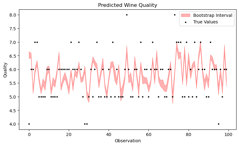
upper = np.percentile(all_preds, 100 * (1 - alpha / 2), axis=0)The plot shows that the resulting bootstrapping bands are very narrow. It's important to note that even though the observations are displayed sequentially, this is not a time series. With time series, the exchangeability assumption is violated, but that doesn't deter us – however, that's a topic for a future article. Moreover, only the first 100 observations are shown here, not the entire prediction dataset, as it would become too cluttered otherwise.
Now, let's calculate the coverage probability.
# Number of matches
matches = [(y_true >= lower[i]) & (y_true <= upper[i]) for i, y_true in enumerate(y_new)]

# Coverage probability
coverage = np.mean(matches)

# Average interval width
avg_interval_width = np.mean(upper - lower)
The coverage probability is at a mere 10% instead of the desired 95%, and the average interval width is at 0.21, which is evidently much too narrow. This confirms that bootstrapping does not guarantee coverage.
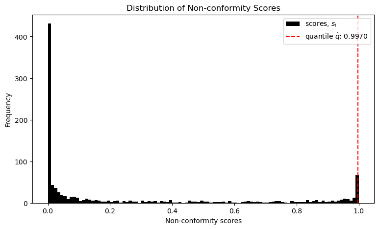
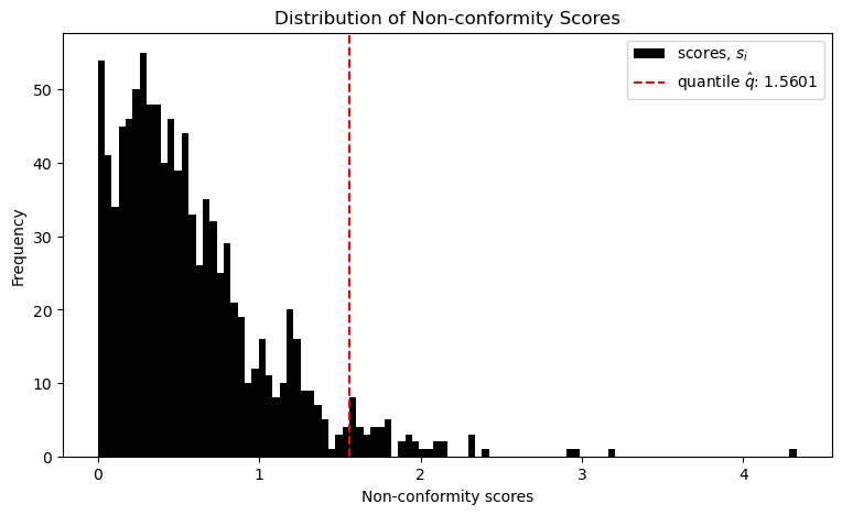
How can Conformal Prediction assist us here? As described above, only the score function needs to be adjusted. In our regression case, it changes as follows, where y is the true value and f is the predicted one. This is just the absolute error.
The other steps remain identical. That means the non-conformity scores s are sorted, and a corresponding 1 − α threshold q is estimated.
# Predicitions
predictions = model.predict(X_calib)

# Non-conformity score
scores = np.abs(y_calib - predictions)

# Error rate
alpha = 0.05

# Quantile
q_level = np.ceil((len(scores) + 1) * (1 - alpha)) / len(scores)

# Treshold
qhat = np.quantile(scores, q_level, interpolation='higher')
The following plot visualizes the result.
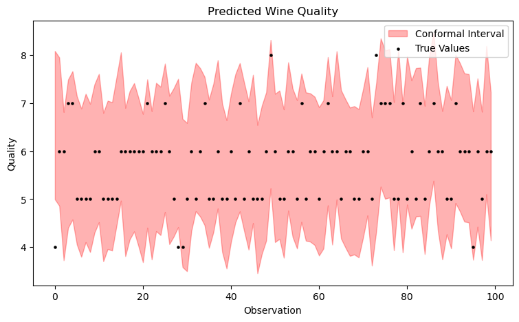
This threshold value q is now both simply added and subtracted from the model's prediction, yielding the prediction intervals.
# Prediction intervals
lower_bounds = []
upper_bounds = []

for i in range(len(X_new)):
    pred = model.predict(X_new[i:i+1])[0]
    lower = pred - qhat
    upper = pred + qhat
    lower_bounds.append(lower)
    upper_bounds.append(upper)

# Coverage probability
matches = [(true_val >= lower) and (true_val <= upper)
           for true_val, lower, upper in zip(y_new, lower_bounds, upper_bounds)]
coverage = np.mean(matches)

# Average interval width
avg_interval_width = np.mean([upper - lower for lower, upper in zip(lower_bounds, upper_bounds)])
The following plot already indicates that the coverage is now significantly better. In fact, this time it is at 97% with an average & constant width of about 3.1. Great!
Of course, this is not yet optimal. For example, the intervals can be designed adaptively rather than constantly, which is accomplished by the Adaptive Conformal Regression Algorithm that uses standardized residuals for its scoring function. However, we won't cover that here.
Conclusion
As we have seen, Conformal Prediction is a broadly applicable technique to generate interval predictions from point predictions, which have guaranteed coverage probability, and which is exceptionally parsimonious with assumptions. This makes it a particularly useful tool that belongs in the repertoire of every statistician, machine learning practitioner and quantitative modeler in general. For more information, literature and application examples, I recommend the following GitHub repository Awesome Conformal Prediction, where this article is featured.
The Code used in this article: